Practical SVBRDF Capture In The Frequency Domain

Code and data

Return to main project page

About

This is a source code and data release for the ACM Siggraph 2013 paper Practical SVBRDF Capture In The Frequency Domain, by Aittala, Weyrich and Lehtinen.

Most of the code is written in Matlab and requires some toolboxes to run (image processing, preferably also parallel toolbox for performance). The capture tool is C++ code and requires the Canon EDSDK. The code is research code, and hence unfortunately is not particularly readable, flexible or efficient. We hope that you will find it useful nevertheless.

License

Copyright (c) 2013-2015 Miika Aittala, Jaakko Lehtinen, Tim Weyrich, Aalto University, University College London. This code and data is released under the Creative Commons Attribution-NonCommercial-ShareAlike 4.0 International license (http://creativecommons.org/licenses/by-nc-sa/4.0/).

Download

Source code (Matlab/C++)
Dataset: Mix (~700 MB)
Dataset: Pynchon (~700 MB)
Dataset: Crumpled (~700 MB)
Dataset: Eco (~700 MB)
Dataset: Tile (~700 MB)
Dataset: Bluebook (~700 MB)
Raw TIFF images for Lindt dataset (3.5 GB)

Contents

The source code archive contains the following directories:

• capture_tool

  C++ source for the software that displays the on-screen patterns and drives the camera. Requires Canon EDSDK.

• optimizer

  MATLAB source for building the dataset from the raw images, specifying calibration, and computing the SVBRDF.

• data

  Placeholder for datasets.

• output

  Placeholder for output data.

Quick start

• Extract the source code archive
• Download all the datasets to the data/ directory
• Run the MATLAB source file COMPUTE_ALL.m
• The solution progress is shown visually, and the solution .mat files will appear in output/ directory

Running the optimizer

The actual optimization is performed by optimizer.m. It shows the current iterate (starting at a low resolution) and gradually improves it. Finally it outputs a Matlab data file sols.mat and the resulting images as 16-bit TIFFs in the specified directory. The displayed images are: diffuse albedo, specular albedo, kurtosis, normals, glossiness, unused (shows upsampling progress), and normals in another visualization. Notice that the glossiness is "inverse" (dark is shiny), as it corresponds to our sigma parameter.

For performance, you should launch a few parallel jobs using matlabpool (if you have it.) The optimizer outputs quite a bit of messy progress data into the console. Thanks to the low-resolution initial stage, you should be able to see rather quickly whether the solution is going to be something reasonable.

    matlabpool 6        
    % Always include the final \ and make sure that the directory exists!
    sols = optimizer(Data, 'Z:\whatever_your_path\mix\'); 

The solution will be in sols, which is a 1024 * 1024 * 10 array. The 10 channels are (for historical reasons): diffuse R, specular R, diffuse GB, specular GB, glossiness, normal x, normal y and kurtosis.

Capture tool

The tool that displays the patterns on the monitor and drives the camera is in the capture_tool/ directory. It is a Visual Studio 2010 project. It also requires the Canon EDSDK for camera control.

Again, this is a crude tool used for research and experimentation. A proper product-like implementation could be significantly more friendly and automated.

We have used a Canon EOS 5D Mk II camera. The temporal syncing between shutter and patterns has been chosen experimentally and may not match the times needed for some other camera model. The important thing is that the shutter must be open by the time the pattern starts showing, and must close after it has finished; preferably with some safety buffer at each end.

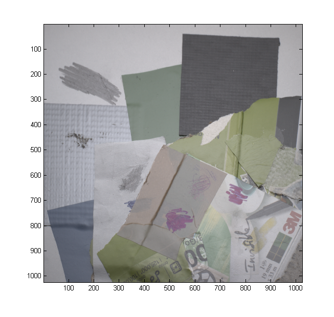
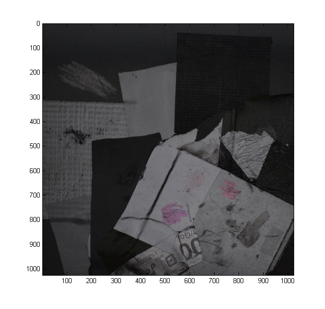
We have included a dataset (Lindt) that contains an entire output of a capture session as TIFF files converted from Canon RAW files by dcraw with maximally linear settings. Have a look at the photos (especially the first ones) to get an idea of what they should look like.

The overall steps for capturing are:

• Place your monitor in a roughly 45 degree downward facing angle. Make sure it is not tilted along any other axis, as the calibration assumes that the monitor x-axis is parallel to the sample plane. Dim the room as much as you can. It does not need to be pitch black; the most important thing is that the lighting conditions do not change during the capture.
• Place the sample under the monitor. Run the capture program. Align the camera so that the reflections from the colored pattern are seen in the region you are interested in. The colored pattern is shown simply for visual aid in aiming. The current implementation only captures square-shaped regions that are aligned with the monitor. It is probably a good idea to use portrait orientation for the camera, because the calibration pattern and the sample need to be visible at the same time and this alignment loses least resolution. We have usually captured our datasets a bit from the side (horizontally), with the assumption that the diffuse and specular lobes may be easier to separate if their centers do not coincide.
• Use the Shoot exposure photo button to find an exposure that is as bright as possible without overexposing any part of the sample. The camera's exposure time must be set to 4 seconds (again, the tool is hardcoded for certain settings; feel free to make a more flexible version.) Shoot RAW images. We've always used a very low ISO number and adjusted the exposure using the aperture (typically something around f/10).
• Next you need to shoot some calibration photos. See the section below for what they should look like. You can shoot them in one combined photo, or two separate photos; what matters is that all the squares are visible in some image. First, you need to place a mirror in place of your sample. Make sure that it is horizontal, and at roughly the same height as your material sample. Use the Shoot calibration photo button. It shows a square on the screen; both the square and its reflection must be visible in the photo.
• The second calibration photo is of a square marker. Simply make a picture of a black square (say, 5-10 cm across) using some paint tool and print it out. Leave some white outside the edges. Place it flat on the mirror, so that it is seen by the camera and roughly aligned with the monitor. Press Shoot marker photo to take a photo of it.
• Finally, put the to-be-captured sample back and press Shoot standard program. The camera will now shoot around 130 photos of frequency patterns, starting with a black frame. It takes around 15 minutes.
• The images are now stored in the camera. Copy them to your disk for processing. If you aligned everything correctly, you should see wave patterns moving across your region of interest when you view the images in sequence.

Calibration tool

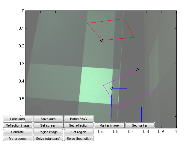
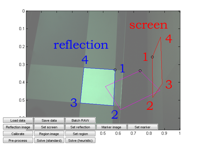
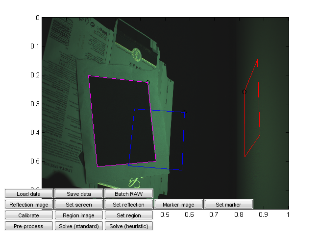
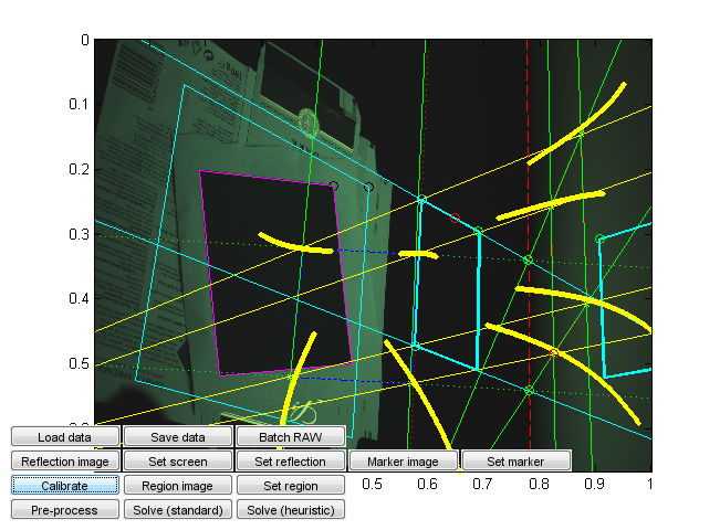
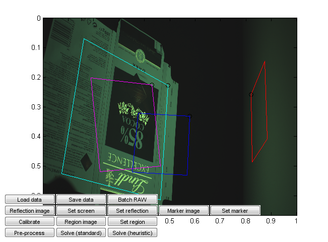
Run calibration_ui.m. This is a calibration and solver launch tool.

This, too, is a crude research tool. Note in particular that it is currently hardcoded assuming a 16:9 capture monitor aspect ratio and a given monitor emission distribution. Change the values from the code if needed. (You can probably recycle the monitor calibration values if they happen to work for you, but the aspect ratio should correspond to that used in the capture.)

The steps are:

• Click Batch RAW and choose any one of your RAW images. This will simply run dcraw with very raw settings for every image in the directory. The output is a huge 16-bit TIFF file for every image. See the console for progress output. (In the attached Lindt dataset, this step is already performed.)
• Click Reflection image and pick the TIFF image that contains the mirror image (IMG_5922.tiff in the example dataset.)
  
• Maximize the window for good clicking accuracy. Click Set screen and then click on each of the corners of the screen square, starting from lower left and advancing counterclockwise (the order is critical.) Try to be accurate. Then click Set reflection and click on the corners of the reflection, in the order that corresponds to the points on the screen. The order is indicated in this image:
  
• Click Marker image and load up the picture that has your black marker in it (IMG_5923.tiff in example.) Click Set marker and pick the corners in clockwise order (starting point does not matter.)
  
• Click Calibrate. This performs the computations in calibrate.m; the output is the geometric configuration. Some information about the geometric construction is drawn on the screen. It might be useful for understanding what the calibration does. The curved yellow lines can be used to determine how successful the calibration was. They should pass through the corners of the screen and reflection squares as seen here:
  
• Click Region image and pick one of the actual frequency data images. Click Set region to choose the area you'll actually want to solve. Do this by first clicking on the upper-left corner of your sample (in "world space") and then the approximate lower right corner. You will see a rectangle that roughly corresponds to your clicks (it must be constrained to a square.) Repeat if it wasn't successful. Make sure no corner of the square is outside the image region.
  

We've also included a button called Solve (heuristic). It simply outputs the magnitude and phase images, and a heuristic guess for the normal map. They could be potentially useful for artists or other purposes.

Exploring the data

The data packages each contain a single .mat file, which contains a Matlab struct. Let us use the Mix dataset as an example. Load it up:

    load('path_to_data\data_mix.mat')

The data will be placed into a struct called Data. To see its contents, simply type Data. The struct contains the image data itself, and all relevant calibration information. For historical reasons, names and conventions do not always match to those in the paper.

Let's first familiarize ourselves with the near-raw data. The instructions for running the actual optimizer are in the end of this section.

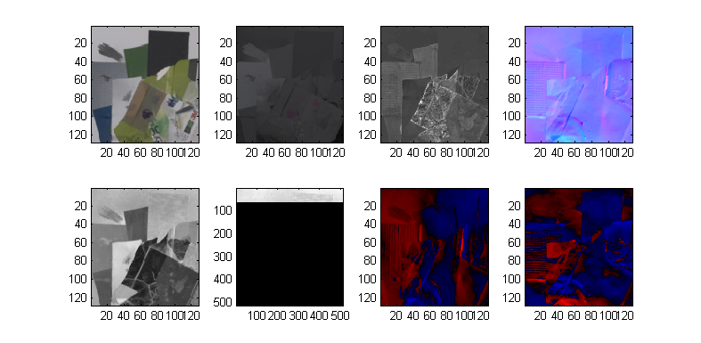
To see the DC component (zeroth frequency image, i.e. simply illuminated by the plain window function), type

    imagec(4*Data.DC);
    

(the factor 4 is just to make it a bit brighter; imagec is our simple color image viewing function which does gamma correction and is a bit less picky than Matlab's image)

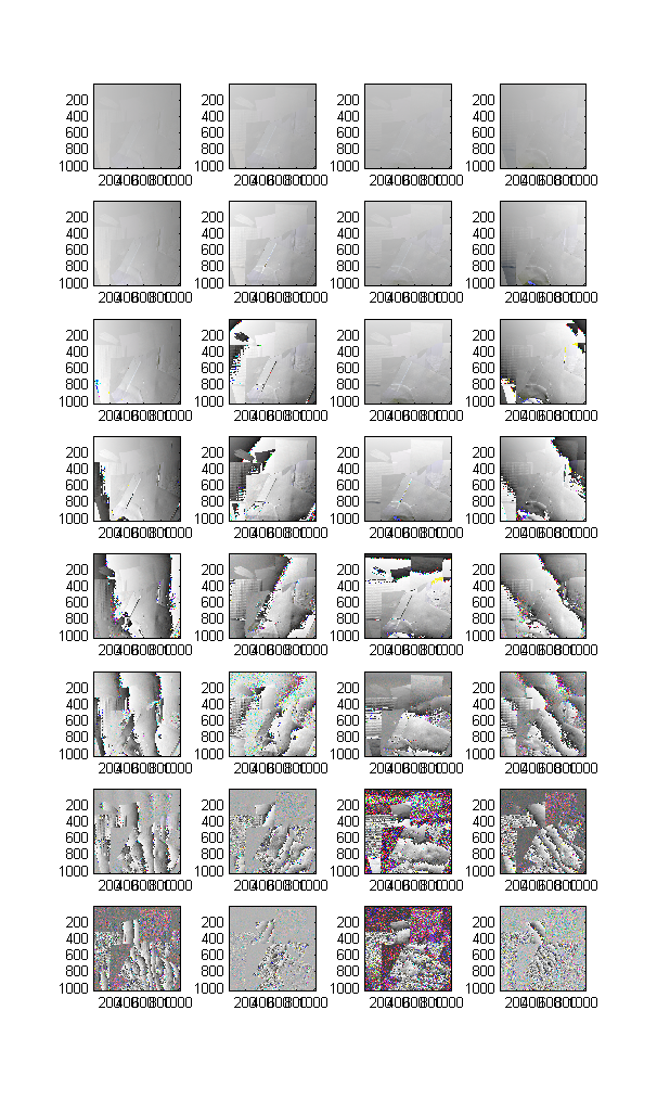
The actual frequency pattern images are stored as complex numbers in Data.Z, which is a 1024 px * 1024 px * 3 colors * 8 frequencies * 4 orientations array. The actual frequencies themselves are listed in Data.freqs. Let's see all the data images at once.

Here are the magnitudes, in a 8*4 array corresponding to orientation and frequency. Notice the effect of increasing frequency: the diffuse component fades away rather quickly.

    % Magnitudes of all data
    clf;
    subplot(8,4,1);
    for o = 1:4
        for f = 1:8
            subplot(8,4,4*(f-1)+o);
            imagec(4*abs(Data.Z(:,:,:,f,o)));  
        end
    end

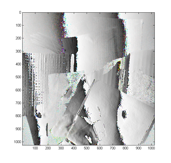
Here's a representative example in higher resolution:

    imagec(4*abs(Data.Z(:,:,:,6,3)));
       

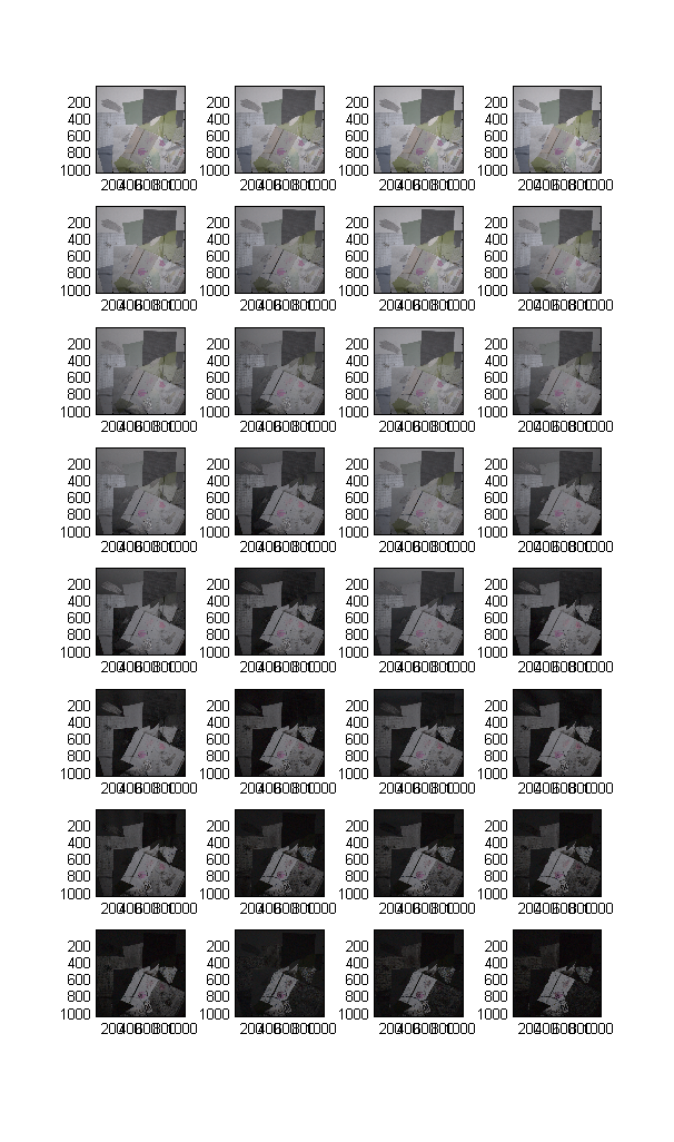
Let's have a similar look at the phase. Clearly the phase seems to contain strong clues about the normals, but it is still distorted especially at low frequencies:

    % Phases of all data
    clf;
    subplot(8, 4,1);
    for o = 1:4
        for f = 1:8
            subplot(8,4,4*(f-1)+o);
            imagec(angle(Data.Z(:,:,:,f,o))/2/pi+0.5);
        end
    end
        

    imagec(angle(Data.Z(:,:,:,6,1))/2/pi+0.5);
        

One could extract quite a bit of useful heuristic information out of this sort of near-raw data itself, if accuracy is not critical and the surfaces are glossy (it is the mixing of diffuse and specular that makes it difficult.) In fact, we base our initial guess on similar reasoning.

Questions, comments

miika_dotaittala_ataalto_dotfi